The Wonderful World of Excel
More than a spreadsheet
Excel is an immensely powerful program for creating, visualizing, organizing, analyzing, and expanding upon datasets both big and small. It is one of the most widely used software applications with hundreds of millions of users. With VBA scripting, you can even program in Excel!
Important!
This module will introduce a fair amount of material, so that you can hit the ground running once the bootcamp starts. Be sure to go through this module, and keep in mind that you will need Excel 2016 to go through these exercises!
Working with cells
Data in Excel is stored in cells. Each cell has an associated row - represented by the numbers on the left side of the application - and column - represented by the letters at the top of the application. Each cell can hold a single piece of data within it, and data can be added into a cell by left-clicking on the cell and then typing in its value. Note that selecting a cell with some data inside of it and then beginning to type will overwrite the original value unless you select the cell and then modify its value in the "formula bar" instead (or double-click the cell).

Excel also allows you to select multiple cells at the same time by left-clicking and then dragging your cursor across the cells you wish to look at. A group of two or more cells is known as a range.
You can select an entire row by clicking a row header at the left of the application.

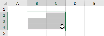
You can fill in multiple cells all at once by selecting a range, left-clicking on the bottom-right corner of the range (this box is called the fill handle), and then dragging the cursor across the range you would like to fill in. Excel automatically fills in the empty range based on the pattern of the original values.

If you would like to add a new row or column between other rows or columns, simply click on the row or column header you would like to insert your data into, right-click, and select "Insert" from the menu that appears.
The formula bar
In order to create a formula, simply left click on the cell you wish to modify and then type in an equals sign.
You can create references to other cells on your spreadsheet by simply clicking on them (or typing their reference - e.g. A2). This will import their value into your new cell. Whenever you change the referenced cell, therefore, the value of the cell containing your formula will also change now.
You can also use mathematical functions to create more complex formulas that take in multiple values. For example, after referencing one cell, you can add a plus sign and then reference a second cell in order to find the sum of both cells.
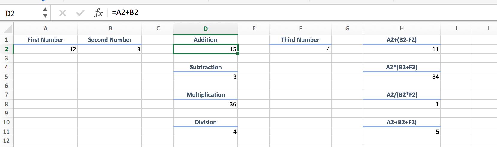
Let's try creating a basic calculator in Excel.
Place two numbers into cells A2 and B2. These values will be those that you use to perform your calculations.
In cell D2, create a formula that adds A2 and B2 together.
In cell D5, create a formula that subtracts B2 from A2.
In cell D8, create a formula that multiplies B2 and A2 together.
In cell D11, create a formula that divides A2 by B2.
Bonus: try creating the formulas required for the cells H2, H5, H8, and H11.
Built-in formulas in Excel
Excel not only includes basic mathematical functions, but also includes built-in functions that allow for more intricate calculations.
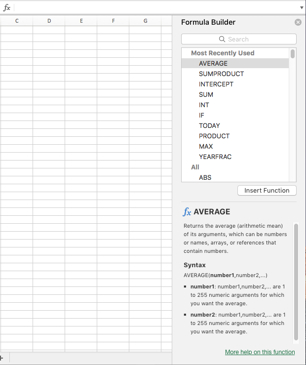
Click on the fx button to the left of the formula bar for a partial list of the built-in functions.
In order to find the sum of a range of values, type in =SUM(<Range>) where <Range> includes the values you wish to add.
To define a range, you can either select with your mouse (click and drag) OR type the beginning and end cells in yourself, separated by a colon (e.g. A1:A10)
In order to find the product of a range of values, type in =PRODUCT(
In order to count how many values are within a range, =COUNT(
Look up MAX() and MIN() functions as well!
Named ranges
Ranges can get somewhat confusing to reference when all of them look like A1:A200 or B3:E20. It would be nice if we could just give these ranges a name, wouldn't it?
Thankfully we can! Whenever we select a cell or a range, we can create a named reference to it by clicking on the cell/range's reference at the top-left of the spreadsheet and then typing in what we would like to name this data.
Try recreating the following worksheet in Excel, then select the range of cells in the column as shown:
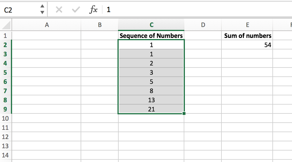
Then click in the cell's reference in the top left corner of the worksheet, as shown, and type in the word "Fibonacci." Next time you select the cells C2:C9, the word "Fibonacci" will be displayed there.
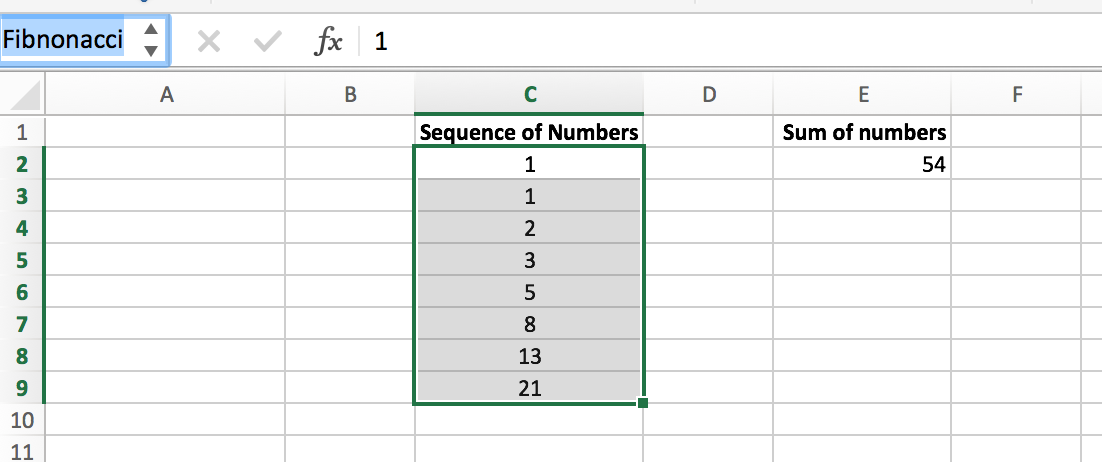
For practice, in cell E2 enter a formula to sum the range C2:C9, then give it a name: "Fibonacci sum."
Conditionals
Sometimes we want to modify our output to return one value if a condition is met and another in the case that it isn't. This is where conditionals in Excel come in.
The IF() function checks whether a particular condition is met by the data sent into it and returns one value if true and another value if false.
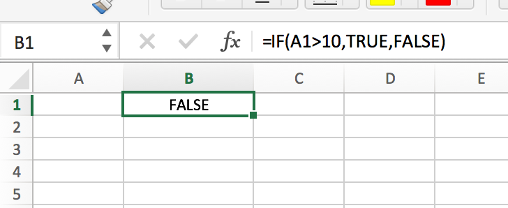
For example, the function =IF(A1>10,TRUE,FALSE) will return the value of "TRUE" if the value of A1 is greater than 10, and it will return "FALSE" if A1 is less than or equal to 10. Let's give it a try.
In B1, enter the above formula and click return:
Now try entering 11 in A1 and press enter:

Excellent (pun intended!). Depending on the value entered in A1, our formula changes the value in A1 to TRUE or FALSE. Let's discuss the formula. We start with =IF(). Easy enough. This part tells us that the value returned in that cell will be a conditional, i.e. it will depend on some condition(s).
What are the three things that go in the parentheses?
The first input is a logic test. This is where we check two or more values against one-another in order to determine whether the statement is true or false. Common symbols that you will find here are
>(greater than),<(less than),=(equal to),<>(not equal to),>=(greater than or equal to), and<=(less than or equal to).The second input is the value we will want to return if the logic test comes back as true. It can be a formula, a string, or an integer.
The third input is similar to the second: it is the value returned if the logic test comes back as false.
Excellent! (The joke never gets old.)
Conditionals, part 2
Now let's try a slightly more complicated example. We'll recreate the worksheet pictured here:
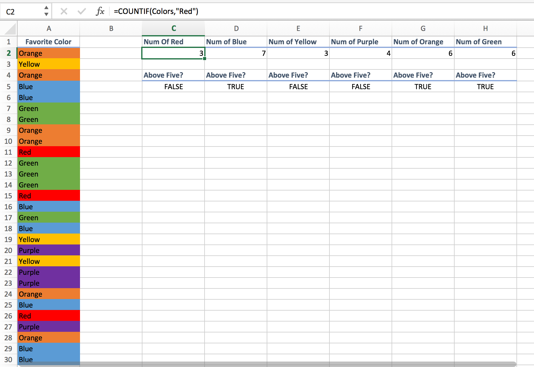
In range A2:A30, enter the following formula: =CHOOSE(RANDBETWEEN(1,6),"Red","Blue","Yellow","Green","Purple","Orange")
Remember that you can enter it once in A2 and drag the lower right corner of the cell down to A30. This formula chooses a random value between 1 and 6, inclusive, then chooses a color whose position corresponds to that number.
Next, give the name "Colors" to the range A2:A30 (see the section of named ranges for how to do this).
In C2, enter the formula =COUNTIF(Colors,"Red"). Do the same for D2:H2. The COUNTIF() function in Excel counts only values that pass the logic test that is contained within its parentheses. This is a shorthand for "count the number of cells in this range that are this value". =COUNTIF(Colors,"Red") checks every cell in the named Colors range and returns the count of how many passed the test.
The conditional formulas for range C5:H5 will be left as an exercise for you. Remember the three inputs required by an =IF() function!
Here's the last, slightly tricky part: we can add one or more conditions with operators such as AND() or OR(). In K5, enter the following formula: =IF(AND(H5,NOT(C5)), TRUE, FALSE) and label it as "Green and Red' in K4.
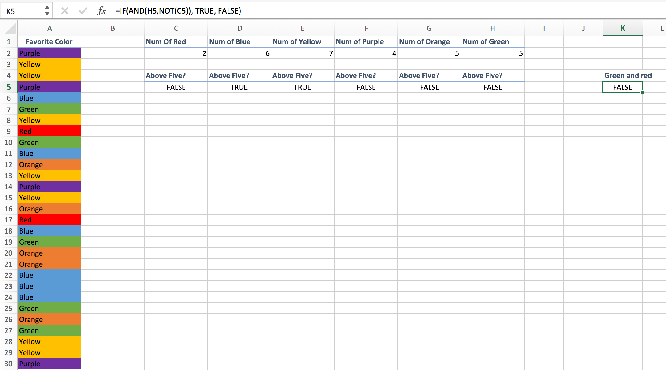
The two conditions are enclosed within the parentheses in AND(). In this instance, K5 will return if the following two conditions are met: H5 is TRUE, and C5 is false. In other words, in AND(H5,NOT(C5), H5 means that H5 returns true, and NOT(C5) means that C5 returns false.